Sim2real ball balancer

Jul – December 2025 · Paused · Reinforcement learning, Isaac Lab, PPO, C++, ONNX, Raspberry Pi

A ball lies on a round plate. Three stepper motors under the plate can tilt it in any direction, and a camera on a mast looks down at it. The task is to keep the ball in the centre, even when someone gives it a push. A classic solution would measure the ball’s position with image processing and run a PID controller on it. This project tries the other route: a neural network that gets nothing but the last four camera images and learns by itself which way to move the motors. It learns in simulation, where a dropped ball costs nothing and 512 copies of the robot train at once, and the trained network is then meant to run on the real robot. That second step, from simulation to reality, is what sim2real refers to.

The policy balances the ball reliably in simulation. On the Raspberry Pi the camera, frame stacking and network inference run, but the loop to the motors is not closed yet. The project is paused until my thesis is finished. The reinforcement learning basics used here are explained in Reinforcement learning fundamentals.

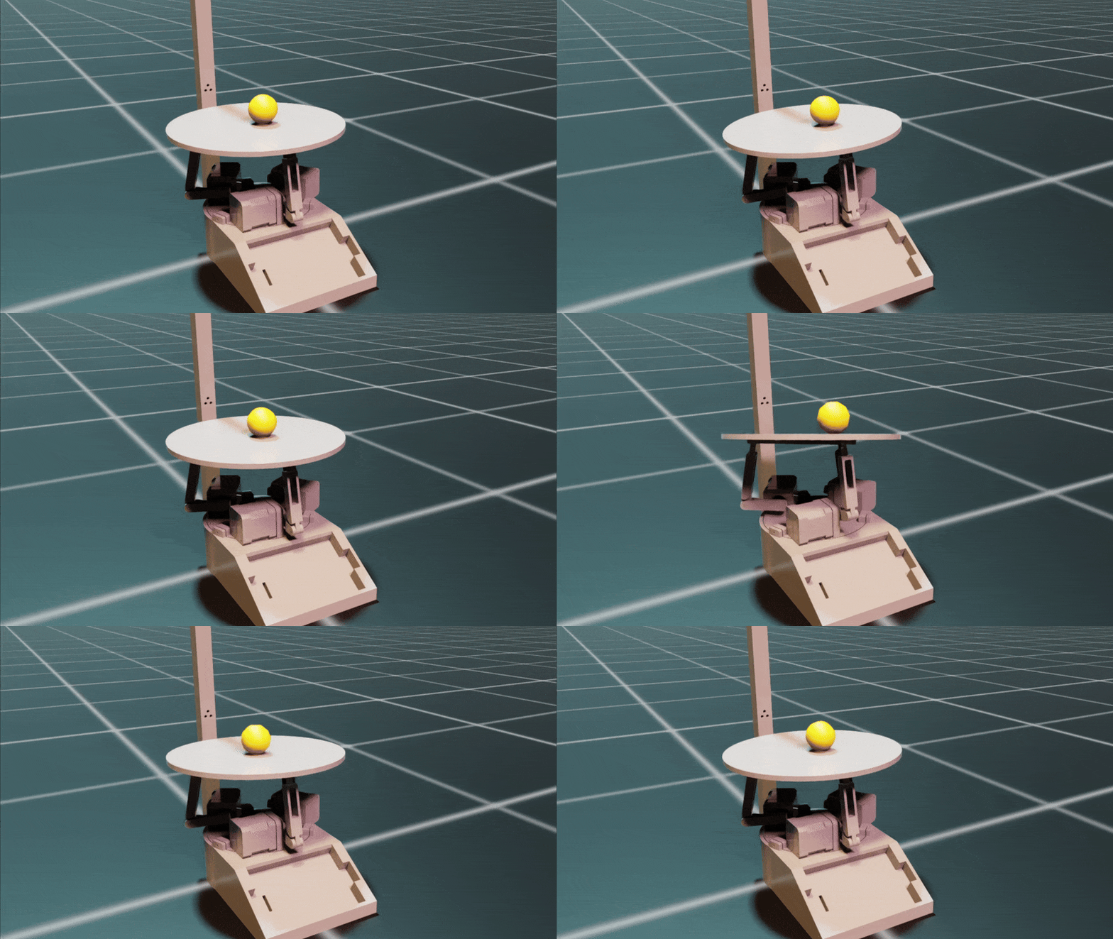Trained agent balancing the ball in simulation Fig. 1: The trained policy balancing the ball in Isaac Lab

The robot

The platform is designed in Fusion 360 and 3D printed. Three NEMA 17 stepper motors sit at 120° around the base. Each one turns a short crank, and a push rod connects the end of the crank to the underside of the plate. When a crank turns up, it lifts its corner of the plate. A mast on the base holds the camera above the plate. The motors are driven by TMC2209 stepper drivers, which take one pulse per step and a direction signal, and a Raspberry Pi generates these pulses on its GPIO pins.

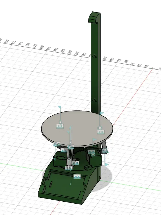The ball balancer in Fusion 360 Fig. 2: The CAD model. Three cranks with push rods carry the plate, the mast holds the camera.

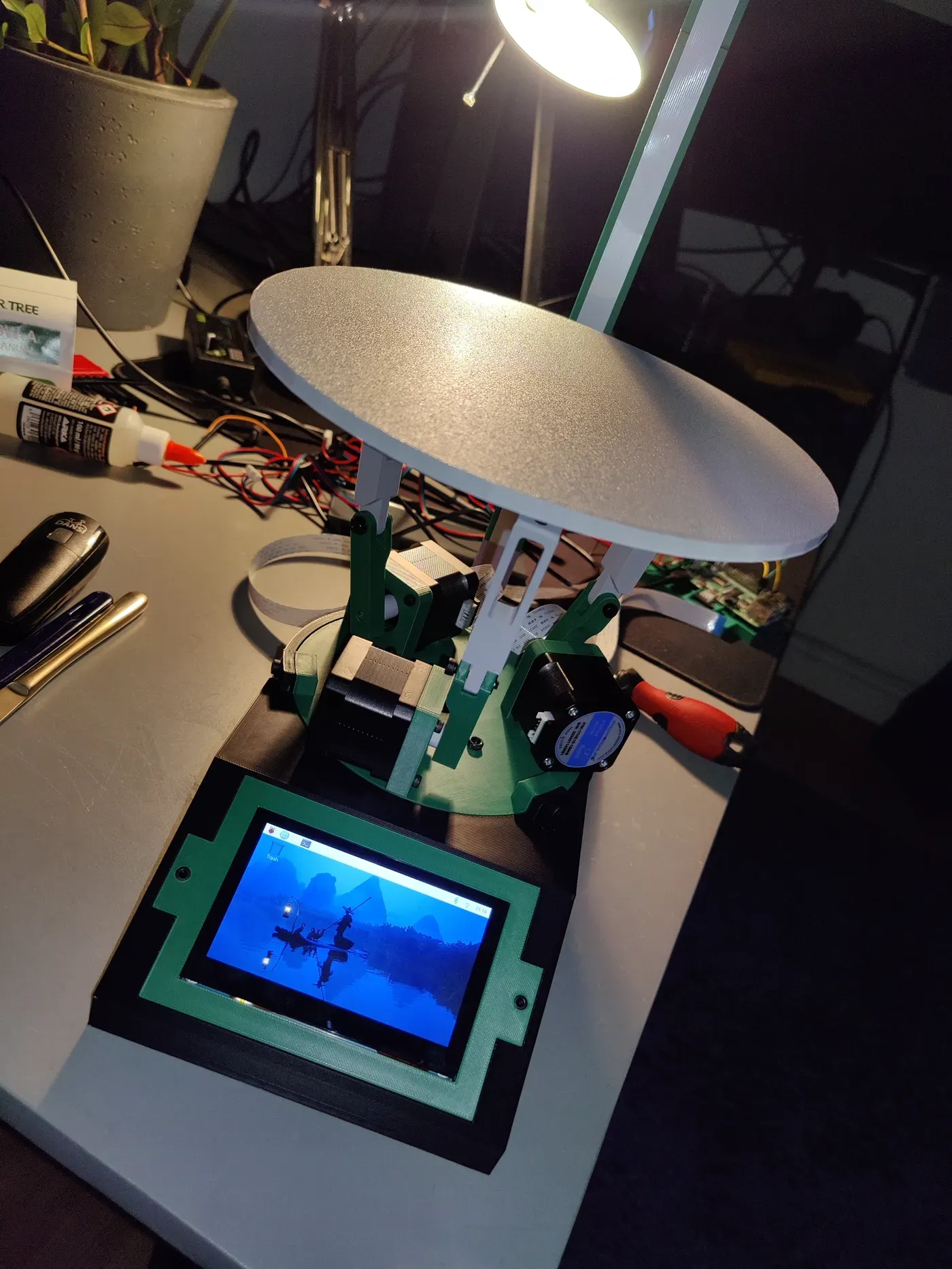The assembled ball balancer on a desk Fig. 3: The assembled robot, here still with a display in the base, which was removed in a later version

From motor angles to tilt. The plate rests on three points, so its height and its two tilt angles are fixed by the three rod heights. For a feel of the geometry, assume the rods meet the plate at radius $r$ and angles $\varphi_i = 90°, 210°, 330°$ , and that crank $i$ with length $L$ at angle $q_i$ lifts its rod by $z_i = L \sin q_i$ . The plate is then the plane $z = z_0 + g_x x + g_y y$ through the three rod ends, with

g_x = \frac{2}{3r} \sum_{i=1}^{3} z_i \cos\varphi_i, \qquad g_y = \frac{2}{3r} \sum_{i=1}^{3} z_i \sin\varphi_i .

The factor $\tfrac{2}{3r}$ comes from $\sum_i \cos^2\varphi_i = \tfrac{3}{2}$ for three points spaced 120° apart. The gradient $(g_x, g_y)$ points uphill, and a ball rolls the other way. A table tennis ball is a thin shell, so part of the energy goes into rotation, and it accelerates with $\tfrac{3}{5} g \sin\theta$ down a slope of angle $\theta$ , a bit less than the $\tfrac{5}{7} g \sin\theta$ of a solid ball. In the actual simulation none of this is hand-coded: the physics engine solves the real linkage from the CAD model. The formula is what the interactive demo below uses.

The environment, step by step

The simulation is a direct environment in NVIDIA Isaac Lab,¹ which runs the physics of many robots in parallel on the GPU and renders a camera image for each of them. One environment step works as follows.

1. Timing. The physics runs at 120 Hz. The policy makes a decision only every 12 physics steps (decimation = 12), so it acts at 10 Hz and each action is held for 0.1 s. An episode lasts 15 s, that is 150 decisions, unless the ball falls off first.

2. Action. The policy outputs three numbers $a_i \in [-1, 1]$ , one per motor. They are not absolute angles but changes of the joint target, at most 0.15 rad per step:

q_i^{\text{target}} = \operatorname{clip}\big(q_i + 0.15\, a_i,\; q_i^{\min},\; q_i^{\max}\big)

def _apply_action(self) -> None:
    limits = self.robot.data.joint_pos_limits[:, self._control_joint_ids]  # (N, 3, 2)
    low, high = limits[..., 0], limits[..., 1]

    current = self.robot.data.joint_pos[:, self._control_joint_ids]       # (N, 3)
    delta = self.cfg.action_scale * self._actions                         # (N, 3)
    targets = torch.clamp(current + delta, min=low, max=high)
    self.robot.set_joint_position_target(targets, joint_ids=self._control_joint_ids)

Relative actions make small corrections easy to learn, because $a = 0$ means “stay where you are”. They also limit how fast the plate can move: 0.15 rad per 0.1 s is at most 1.5 rad/s per motor.

3. Observation. A simulated camera above the plate renders a 64 × 64 RGB image. The policy sees the last four of them, stacked along the colour channels into one tensor of shape 12 × 64 × 64 with values in $[0, 1]$ , newest frame first. A single image shows where the ball is but not where it is going. Four images 0.1 s apart also show its velocity, and that is enough to make the problem Markov again. The joint angles are deliberately not part of the observation. The config keeps them commented out, with my note from back then:

# stabilzes training a lot and yields far better results. However the real robot only has a camera
# "joints": spaces.Box(low=-1.0, high=1.0, shape=(3,), dtype=np.float32),

4. Reset and disturbances. Every episode starts with the ball released just above the plate, at a random position in a 10 cm × 10 cm square around the centre. It gets a random initial velocity of up to 0.6 m/s, aimed roughly at the centre (within ±30°), so the policy has to catch it. During the episode, every 2 to 8 s, the ball gets a random kick: up to 0.6 m/s more velocity in a random direction plus a random spin of up to 10 rad/s per axis. A policy that only learned to keep a resting ball still would fail at the first kick.

5. Reward. With $d$ the distance of the ball from the centre in metres, $v$ its speed in m/s and $q_i$ the joint angles in radians, every step that the ball stays on the plate earns

r = 1 + 0.5\, b - 10\, d^2 - v^2 - w \sum_{i=1}^{3} q_i^2, \qquad b = \frac{\max(0.01 - d,\; 0)}{0.01}.

The terms, one by one:

Term	Meaning
$1$	staying alive. Every step on the plate is worth something.
$0.5\, b$	centre bonus, up to 0.5, falls linearly to 0 at 1 cm from the centre
$-10\, d^2$	keep the ball near the centre
$-v^2$	keep the ball slow
$-w \sum q_i^2$	keep the plate level. $w = 0.02$ , but $w = 0.1$ once the ball is stable: closer than 2 cm and slower than 5 cm/s.

A ball whose centre falls below 5 cm height has dropped off the plate. That step gives $r = -20$ and ends the episode. The higher joint penalty for a stable ball stops the policy from holding the plate at an angle once the job is done.

pos_cost = torch.sum(rel_ball_pos_xy * rel_ball_pos_xy, dim=-1)
vel_cost = torch.sum(rel_ball_vel_xy * rel_ball_vel_xy, dim=-1)
dist, speed = torch.sqrt(pos_cost + 1e-8), torch.sqrt(vel_cost + 1e-8)

is_stable = (dist < 0.02) & (speed < 0.05)
joint_penalty = torch.where(is_stable, 0.1, 0.02)
tilt_cost = torch.sum(joint_pos * joint_pos, dim=-1) * joint_penalty

center_bonus = torch.clamp(0.01 - dist, min=0.0) / 0.01
reward = 1.0 + 0.5 * center_bonus - 10.0 * pos_cost - 1.0 * vel_cost - tilt_cost
reward = torch.where(dropped, -20.0 * torch.ones_like(reward), reward)

Interactive demo

The demo below is a 2D version of the environment, seen from above. Timing, action interface, spawn, kicks and reward are the same as in the Isaac Lab environment. The plate size, joint range and crank geometry are rough values, and the ball rolls on the ideal plane from the formula above. Instead of the trained network, either a hand-tuned PD controller or you control the plate. Both act through the same interface as the policy: three relative actions per decision, at most 0.15 rad each.

Training

The policy is trained with PPO² from the skrl library,³ with 512 environments in parallel on one GPU. Policy and value function share one small convolutional network in the style of the Atari DQN and have separate output layers:

Layer	Output for one observation
input: 4 stacked RGB frames	12 × 64 × 64
conv 8 × 8, stride 4, 32 filters, ELU	32 × 15 × 15
conv 4 × 4, stride 2, 64 filters, ELU	64 × 6 × 6
conv 3 × 3, stride 1, 64 filters, ELU	64 × 4 × 4 = 1024
fully connected, ELU	256
output	3 action means (policy), 1 value (value function)

The policy part has 357,539 parameters. The policy is Gaussian: during training, actions are sampled around the predicted means with a learned standard deviation, and for deployment only the means are used.

Each PPO update collects 32 steps from all 512 environments, that is 16,384 transitions, and then runs 8 epochs over them in 8 mini-batches. Discount factor $\gamma = 0.99$ , GAE $\lambda = 0.95$ , clip ratio 0.2, learning rate $5 \cdot 10^{-4}$ with a scheduler that adapts it to the KL divergence between old and new policy. Rewards are scaled by 0.1 before PPO sees them. The configured run is 1,200 steps per environment, 37 PPO updates and about 614,000 transitions in total, which corresponds to 17 hours of simulated balancing.

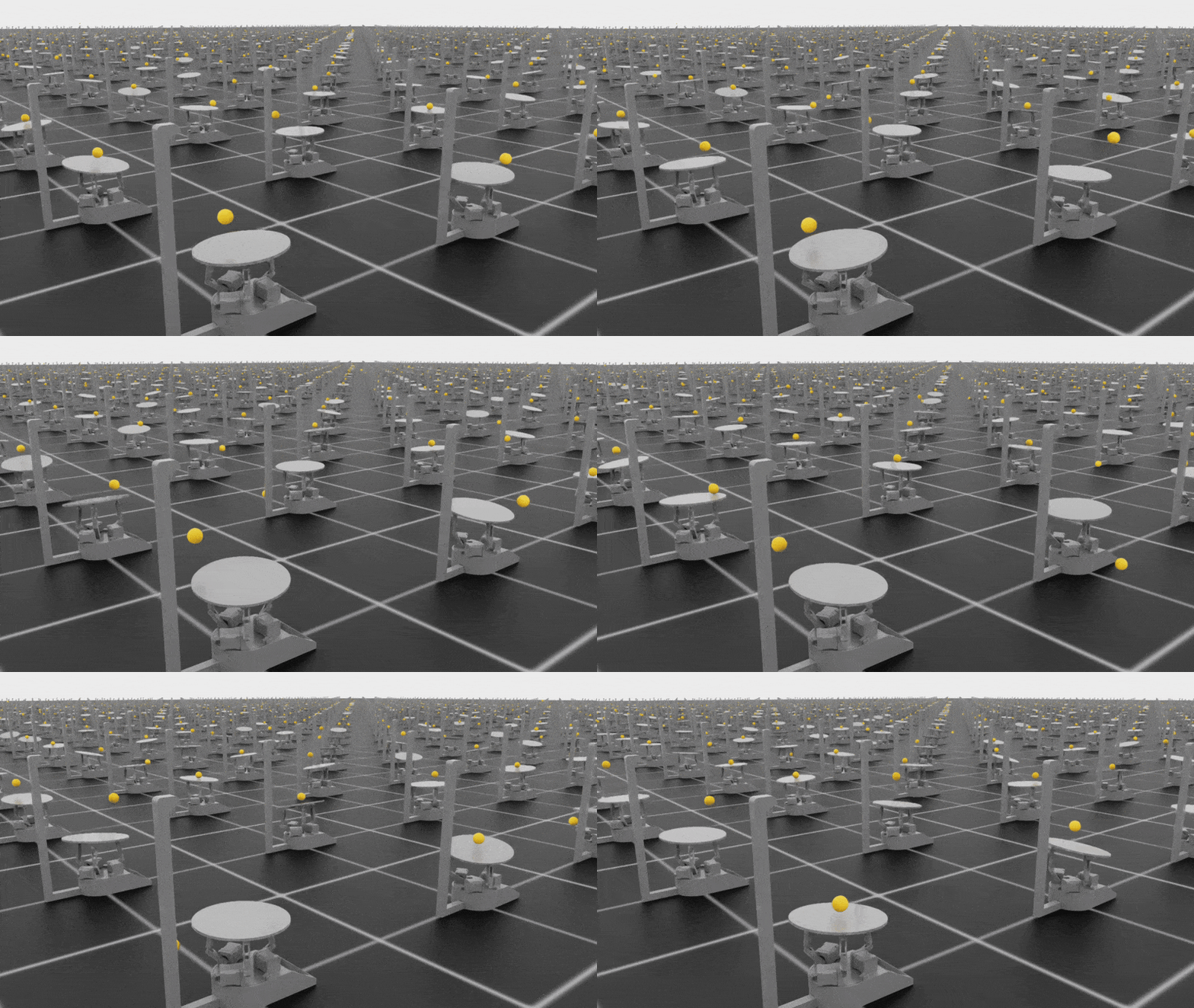The start of training in 512 parallel environments Fig. 4: The start of training. 512 copies of the robot, most balls fall off within seconds.

The simulated robot has to match the real one. The USD model is exported from the same Fusion 360 design, and driving the simulation and the real motors with the same commands side by side shows whether joint directions and zero positions agree.

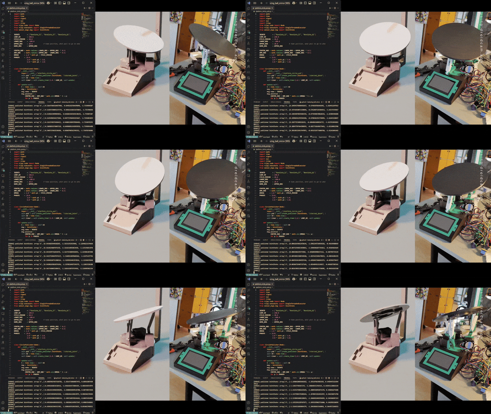Simulation and real robot moving in sync Fig. 5: Digital twin. The simulation and the real robot rotate the platform in sync.

On the Raspberry Pi

After training, the policy is exported to ONNX and run on the Raspberry Pi in C++ with ONNX Runtime. The pipeline mirrors what the policy saw in simulation:

Capture. libcamera delivers 1920 × 1080 frames at 30 fps, with fixed exposure (15 ms) and gain, so the brightness does not drift while the ball moves.
Crop and scale. The centre square of the frame is cut out and scaled down to 64 × 64.
Stack. A queue keeps the last four frames, newest first. On the first call the same frame is repeated four times, exactly as the environment does after a reset.
Convert. BGRA becomes RGB, the bytes become floats in $[0, 1]$ , and the four frames are rearranged into the 12 × 64 × 64 layout of the training tensor.
Infer. ONNX Runtime with four threads computes the three action means, then the loop waits 100 ms, for roughly the 10 Hz of the simulation.

cv::Mat getNextFrameStack()
{
    cv::Mat frame = cam_.getFrame();
    cv::Mat resized;
    cv::resize(cropCenterSquare(frame), resized, cv::Size(width_, height_), 0, 0, cv::INTER_LINEAR);

    if (!initialized_) {                     // first call: repeat the frame four times
        for (int i = 0; i < 4; ++i) frames_.push_front(resized.clone());
        initialized_ = true;
    } else {                                 // newest frame left, drop the oldest
        frames_.push_front(resized.clone());
        if (frames_.size() > 4) frames_.pop_back();
    }
    cv::Mat stack;
    cv::hconcat(std::vector<cv::Mat>(frames_.begin(), frames_.end()), stack);
    return stack;
}

The motors have their own driver. Each motor gets a worker thread that toggles the step pin, with 100 µs high and 100 µs low per step by default. With 16× microstepping a revolution has $200 \cdot 16 = 3200$ steps of 0.1125°, so the motor turns at most $5000 \cdot 0.1125° = 562.5°/\text{s}$ . A new command interrupts a running move, so the motor always heads for the latest target. A position controller on top converts target angles into step counts relative to the counted position. It was tested with a small command-line tool and a random agent that sends new targets at 10 Hz.

For later, the repository also contains the first policy version compiled for a Hailo AI accelerator for the Raspberry Pi, and a test program that runs a single inference on it. Quantization and using it in the control loop are still open on the roadmap.

Status

What works:

The Isaac Lab environment, training, and a policy that balances the ball from pixels
The digital twin, the stepper driver, and camera capture with frame stacking on the Pi
ONNX inference on the Pi on live camera images

What is missing is the last connection: main.cpp computes the actions and prints them, but does not send them to the motors yet. So the real robot has not balanced a ball.