Handwritten digit recognizer in C++

Libraries like PyTorch make a neural network a few lines of code. That is convenient, but it also hides everything interesting: what a neuron computes, where the gradients come from and why training works at all. For this project I wrote a small neural network in plain C++, with no ML library, and trained it to read handwritten digits. A second program opens a window where you draw a digit with the mouse and see what the network thinks it is.

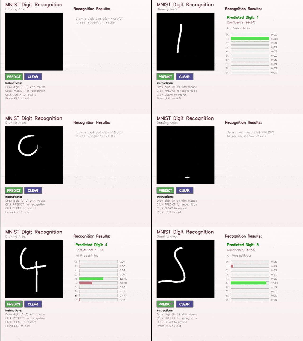Drawing app with live digit recognition Fig. 1: The drawing app. The bars on the right are the network’s probabilities for the ten digits.

The repository has three parts: mlp, a small library with the network itself, MNIST, which trains and evaluates it, and draw_and_predict, the drawing app.

The data

MNIST¹ is the classic dataset for this task: 70,000 grayscale images of handwritten digits, 28 × 28 pixels each, split into 60,000 training and 10,000 test images. I used the CSV version, where every row is the label followed by 784 pixel values from 0 to 255.

The network does not see an image, it sees a list of 784 numbers. Each pixel is scaled to $[0, 1]$ , and the label becomes a one-hot vector: ten numbers that are all 0 except a 1 at the position of the correct digit. A 3 becomes $(0, 0, 0, 1, 0, 0, 0, 0, 0, 0)$ . That is the shape the network’s output should have.

std::vector<double> oneHotEncode(int label, int numClasses = OUTPUT_SIZE)
{
    std::vector<double> encoded(numClasses, 0.0);
    encoded[label] = 1.0;
    return encoded;
}

The 60,000 training images are split once more: the first 48,000 are used for training, the last 12,000 for validation, i.e. for deciding when to stop training. The test set is only used at the very end.

One neuron

The building block is a single artificial neuron, the Perceptron class. It has one weight $w_i$ per input and a bias $b$ . It multiplies every input by its weight, adds everything up and passes the sum through an activation function:

z = \sum_{i} w_i x_i + b, \qquad a = \sigma(z) = \frac{1}{1 + e^{-z}}

The sigmoid $\sigma$ squashes any number into $(0, 1)$ . A large positive $z$ gives almost 1 (“the neuron fires”), a large negative one almost 0. A weight says how much an input matters and in which direction: positive weights vote for firing, negative ones against.

double Perceptron::calcOutputRaw(const std::vector<double> &inputs) const
{
    double sum = m_bias;
    for (size_t i = 0; i < inputs.size(); i++)
        sum += m_weights[i] * inputs[i];
    return sum;
}

double Perceptron::activate(double x) const
{
    return 1.0 / (1.0 + std::exp(-x));
}

One neuron can only separate its inputs with a straight line (a hyperplane, in 784 dimensions). That is not enough to tell a 4 from a 9.

From neurons to a network

The trick is to stack neurons in layers, where every layer reads the outputs of the one before. The network here has two hidden layers:

\underbrace{784}_{\text{pixels}} \;\to\; 128 \;\to\; 64 \;\to\; \underbrace{10}_{\text{digits}}

Writing all weights of a layer as a matrix, with one row per neuron, the whole forward pass is three lines:

\begin{aligned} h_1 &= \sigma(W_1 x + b_1) && W_1 \in \mathbb{R}^{128 \times 784} \\ h_2 &= \sigma(W_2 h_1 + b_2) && W_2 \in \mathbb{R}^{64 \times 128} \\ p &= \operatorname{softmax}(W_3 h_2 + b_3) && W_3 \in \mathbb{R}^{10 \times 64} \end{aligned}

That makes $100{,}352 + 8{,}192 + 640$ weights and $128 + 64 + 10$ biases, 109,386 parameters in total. The hidden layers learn their own intermediate features. Nobody tells them to look for loops or strokes, training finds whatever helps.

The output layer has no sigmoid. Its ten raw scores $z$ , the logits, go through a softmax instead, which turns them into probabilities that are positive and sum to 1:

p_k = \frac{e^{z_k}}{\sum_{j=1}^{10} e^{z_j}}

The predicted digit is simply the one with the largest $p_k$ . In the code a layer is a std::vector<Perceptron>, and the forward pass loops over the layers:

std::vector<double> MLP::forward(const std::vector<double> &inputs)
{
    std::vector<double> activations = inputs;
    for (const auto &hiddenLayer : m_Layers->hiddenLayers)
        activations = computeLayerOutput(hiddenLayer, activations, false); // with sigmoid
    return applySoftmax(computeLayerOutput(m_Layers->outerLayer, activations, true));
}

applySoftmax subtracts the largest logit before calling exp. This does not change the result, because the factor $e^{-\max z}$ cancels in the fraction, but it keeps exp from overflowing for large logits.

Try it

The demo below runs the trained network from the repository in your browser. It is the same forward pass as above, with the weights exported from the model file.² Draw a digit in the left box, or pick one of the MNIST test images.

Learning: loss and gradients

At the start all weights are random, so the output is random too. Training means changing the weights until the outputs match the labels. For that we need a number that says how wrong the network is, the loss. For softmax outputs the natural choice is the cross-entropy between the prediction $p$ and the one-hot label $y$ :

L = -\sum_{k=1}^{10} y_k \log p_k = -\log p_{\text{correct}}

If the network gives the correct digit probability 1, the loss is 0. If it gives it 0.01, the loss is $-\log 0.01 \approx 4.6$ .

To reduce the loss we need to know, for every single weight, in which direction to change it. That is the gradient $\partial L / \partial w$ , and backpropagation³ computes all 109,386 of them in one sweep from the output back to the input, using the chain rule.

Output layer. Softmax and cross-entropy fit together very nicely. If you work through the derivative of $L$ with respect to the logits $z$ , almost everything cancels:

\delta_3 = \frac{\partial L}{\partial z_3} = p - y

The error signal of an output neuron is simply “predicted minus wanted”. If the network said 0.7 for the correct digit, that neuron gets $-0.3$ . A wrong digit that got 0.2 gets $+0.2$ .

Weights. A weight $w_{ki}$ connects input $a_i$ to neuron $k$ . Since $z_k = \sum_i w_{ki} a_i + b_k$ , its gradient is the neuron’s error times the input that flowed through it, and for the bias just the error:

\frac{\partial L}{\partial w_{ki}} = \delta_k \, a_i, \qquad \frac{\partial L}{\partial b_k} = \delta_k

Hidden layers. A hidden neuron has no label of its own. Its error is collected from the neurons it feeds into, weighted by the connecting weights, and then scaled by the slope of its sigmoid. The sigmoid has the convenient derivative $\sigma'(z) = \sigma(z)\,(1 - \sigma(z))$ , so the slope can be computed from the activation alone:

\delta_2 = \left(W_3^\top \delta_3\right) \odot h_2 \odot (1 - h_2), \qquad \delta_1 = \left(W_2^\top \delta_2\right) \odot h_1 \odot (1 - h_1)

$\odot$ is element-wise multiplication. This is where the name comes from: the errors travel backwards through the same weights the activations travelled forward through.

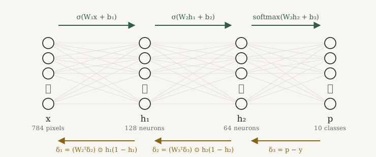Forward and backward pass through the network Fig. 2: The forward pass computes the activations from left to right. The backward pass sends the error signals δ from right to left through the transposed weights.

Update. Finally, every weight takes a small step against its gradient. The step size $\eta$ is the learning rate, 0.01 here:

w_{ki} \leftarrow w_{ki} - \eta\, \delta_k\, a_i, \qquad b_k \leftarrow b_k - \eta\, \delta_k

In the code the three steps look like this (shortened from MLP::train):

// output layer: softmax + cross-entropy gives (output - target)
for (size_t i = 0; i < outerLayer.size(); i++)
    outputDeltas[i] = softmaxOutputs[i] - targets[i];

// hidden layer: collect the error from the next layer, times the sigmoid slope
double error = 0.0;
for (size_t k = 0; k < nextLayer.size(); k++)
    error += nextLayer[k].getWeights()[i] * nextDeltas[k];
currentDeltas[i] = error * currentActivations[i] * (1.0 - currentActivations[i]);

// every neuron updates its own weights
void Perceptron::updateWeights(const std::vector<double> &inputs, double delta)
{
    for (size_t i = 0; i < m_weights.size(); i++)
        m_weights[i] -= m_learningRate * delta * inputs[i];
    m_bias -= m_learningRate * delta;
}

Training

Training uses plain stochastic gradient descent with a batch size of one: forward pass, backward pass and weight update for every single image, 48,000 times per epoch. After each epoch the network is evaluated on the 12,000 validation images. If the validation accuracy has not improved by at least 0.1 percentage points for 5 epochs in a row, training stops early, at the latest after 100 epochs. The validation images are never used for weight updates, so they show how well the network does on digits it has not memorised.

All weights and biases start uniformly random in $[-1, 1]$ . The trained model is written to a binary file: for every neuron the number of weights, the weights, the bias and the learning rate, as raw doubles.

Results

The README reports 96.48 % accuracy on the 10,000 test images, for the version trained with softmax and early stopping. The model file committed to the repository is an older one: it was trained in February 2025 on all 60,000 training images, with a sigmoid output layer and a squared-error loss, before softmax and the validation split were added. I re-evaluated that file on the same test set and got 96.29 %. The demo above uses this file. The per-digit numbers are close:

Digit	README	Committed model	Test images
0	98.37 %	98.47 %	980
1	98.59 %	98.50 %	1,135
2	95.54 %	96.03 %	1,032
3	96.34 %	95.45 %	1,010
4	96.44 %	96.44 %	982
5	94.73 %	94.96 %	892
6	96.35 %	97.29 %	958
7	96.69 %	95.82 %	1,028
8	96.10 %	94.97 %	974
9	95.24 %	94.65 %	1,009
all	96.48 %	96.29 %	10,000

For a network with no convolution and no tricks this is a typical result. The mistakes make sense: the most frequent confusions of the committed model are 4 → 9 (18 times), 9 → 4 and 7 → 9 (15 each) and 3 ↔ 5. Those are pairs that differ by one short stroke.

Two more measurements with the committed model say more about its limits than the accuracy does:

It is overconfident. On the 371 test images it gets wrong, the median probability it gives to its wrong answer is 89 %. A softmax output is a score, not a calibrated probability.
It does not handle shifts. Moving every test image right by 1 pixel drops the accuracy to 92.8 %, by 2 pixels to 73.4 %, by 3 pixels to 47.9 %. Re-centring the test images by their bounding box, the way the drawing app centres a drawing, gives 78.5 %. A fully connected network learns every pixel position separately.

Y. LeCun, L. Bottou, Y. Bengio and P. Haffner, Gradient-Based Learning Applied to Document Recognition, Proceedings of the IEEE, 1998. The CSV version used here is from pjreddie.com. ↩
To keep the download small (120 KB), each weight is stored as an 8-bit integer with one scale factor per layer. On the 10,000 test images this copy agrees with the original double model on 99.87 % of the predictions. The 16 example digits are from the MNIST test set. ↩
D. E. Rumelhart, G. E. Hinton and R. J. Williams, Learning Representations by Back-Propagating Errors, Nature 323, 1986. ↩