Deep Q-learning on Atari Breakout

The next step after the tabular experiments: the same Q-learning update, but the state is no longer one of 16 tiles. It is the screen of an Atari 2600. The agent sees only pixels and the score, and it has to work out by itself what the ball and the paddle are and that hitting the ball pays off. The method is DQN from Mnih et al.,¹ written from scratch in PyTorch. The game comes from Gymnasium and the Arcade Learning Environment.

Video 1: The trained agent with its state value and action values for every step.

From a table to a network

In Frozen Lake the Q-table had 16 × 4 entries. In Breakout a state is an image, and almost no image ever appears twice, so a table is out of the question. Instead a neural network takes the screen and outputs one Q-value per action:

s \;\longmapsto\; Q(s, \cdot\,; \theta) = \big(Q(s, \text{NOOP}),\; Q(s, \text{FIRE}),\; Q(s, \text{RIGHT}),\; Q(s, \text{LEFT})\big)

The outputs are not probabilities. Each is an estimate of the discounted points still to come if the agent presses that button and plays well afterwards. The policy is still $\arg\max_a Q(s, a)$ with ε-greedy exploration, and the state value is simply $V(s) = \max_a Q(s, a)$ . The network is a row of the Q-table that is computed instead of looked up, and it can generalize: similar screens get similar values.

The update is the one from Frozen Lake, with the table cell replaced by the network’s weights $\theta$ :

y = r + \gamma\,(1 - d)\, \max_{a'} Q(s', a'; \theta^-), \qquad \theta \leftarrow \theta - \eta\, \nabla_\theta \big(Q(s, a; \theta) - y\big)^2

$d$ is 1 if the episode ended after this step, and $\theta^-$ are the weights of the target network described below. Done naively, this is unstable. The two tricks that made DQN work, the replay buffer and the target network, both come from one fact: in a network, all states share the same weights.

What the agent sees

The raw screen is 210 × 160 RGB at 60 frames per second. Before the network sees it, the standard DQN preprocessing is applied:

Step	What	Why
Frame skip	repeat each action for 4 frames	4× fewer decisions, the screen barely changes per frame
Max over 2 frames	maximum of the last two frames	the Atari draws some objects only every other frame
Grayscale, 84 × 84	color dropped, image squashed	a third of the data, color carries no information here
Frame stack	the last 4 frames form the state	one image shows where the ball is, four show where it is going
Reward clipping	reward → sign(reward)	the same scale for every game
Life loss = terminal	losing a life ends the episode for learning	see below
Fire on reset	press FIRE after a reset	otherwise Breakout waits forever for the ball to be launched

The frame stack is the Markov property in practice. A single image does not say whether the ball is rising or falling, so the future would depend on the history. Four stacked frames fold that history back into the state.

Treating a lost life as the end of an episode turned out to matter. The target for the last step before losing the ball becomes $y = r = 0$ , a clear signal that this situation is worth nothing. Without it the target would bootstrap from the next life, which is worth almost as much, and losing a ball would look nearly free.

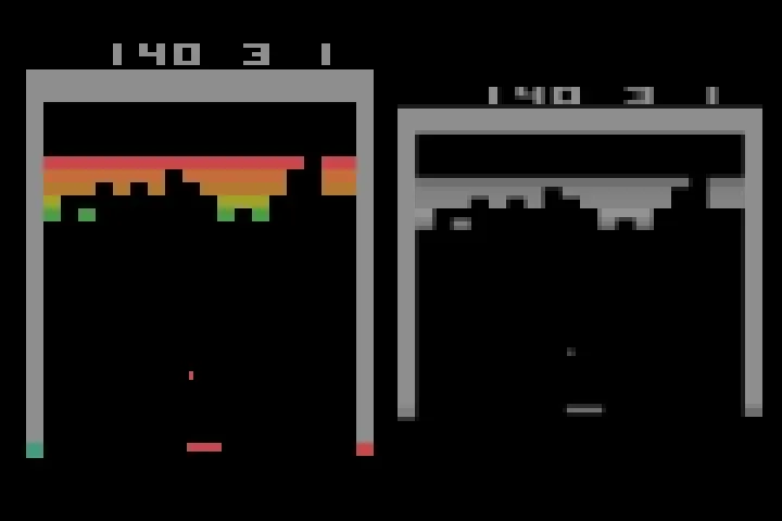The original screen next to the 84 × 84 grayscale frame the network sees Fig. 1: The same moment as the player sees it and as the network sees it. A tunnel has formed on the right.

The network

The CNN from the paper: three convolutions, then two fully connected layers, about 1.7 million weights.

Layer	Output shape
Input: 4 stacked frames	4 × 84 × 84
Conv 8 × 8, stride 4, 32 filters, ReLU	32 × 20 × 20
Conv 4 × 4, stride 2, 64 filters, ReLU	64 × 9 × 9
Conv 3 × 3, stride 1, 64 filters, ReLU	64 × 7 × 7
Flatten, fully connected, ReLU	512
Fully connected	4 Q-values

Each spatial size follows from $(\text{in} - \text{kernel}) / \text{stride} + 1$ , for example $(84 - 8)/4 + 1 = 20$ . The four frames enter as four channels, like the red, green and blue channels of a photo. One filter of the first layer is a block of 4 × 8 × 8 weights, one 8 × 8 slice per frame. At each position the products of all four slices are summed into a single number:

\text{out}(x, y) = b + \sum_{c=1}^{4} \sum_{i=1}^{8} \sum_{j=1}^{8} w_{c,i,j}\; \text{frame}_c(4x + i,\, 4y + j)

Because one filter sees all four frames at once, it can respond to motion: positive weights where the ball is now, others where it was a moment ago. The layer has 32 such filters, so its weight tensor has the shape 32 × 4 × 8 × 8.

Replay buffer

Learning directly from the step that just happened works for a table, because an update to one cell leaves all other cells alone. In a network every update moves all weights, and consecutive Breakout frames are almost identical. Trained on them in order, the network fits the current situation and forgets the others.

So every transition $(s, a, r, s', d)$ goes into a ring buffer of the last 100 000 steps, and the network learns from random minibatches of 32 drawn from the whole buffer. Acting and learning are decoupled: the game only collects data, every gradient step uses data from the buffer.

Mixing. A minibatch contains moments from many different games, which is what gradient descent needs.
Reuse. One minibatch every 4 steps means each transition is used about 8 times before it is overwritten.
Re-evaluation. A stored transition is a fact that stays true: in $s$ , action $a$ led to $r$ and $s'$ . Only the estimate of $s'$ changes. Drawn again later, the same old fact gives a better target, because the network now knows more about $s'$ .

This only works because Q-learning is off-policy. The transitions were collected by older, worse versions of the agent. The target $r + \gamma \max_{a'} Q(s', a')$ asks what $a$ is worth if the agent plays optimally from $s'$ on, and does not care which policy chose $a$ . SARSA’s target contains the action the old policy actually took next, so it would learn the value of an outdated policy.

Target network

The target is computed by the network that is being trained. Since $s$ and $s'$ look almost the same, raising $Q(s, a)$ also raises $Q(s', \cdot)$ , and with it the target. The network chases a goal that moves with every step.

The fix is a frozen copy for the targets, updated every 1000 steps. Between two copies the online network solves an ordinary regression problem with fixed labels. This is value iteration from dynamic programming: compute the new values from the old ones, then replace the old ones. The copy is always slightly out of date, and that is the point.

The first target network is random, and the online network still learns. The new information never comes from the target network. It comes from $r$ and $d$ in the buffer. For a step that ends the episode the target is exactly $r$ , whatever the target network says. From there each round carries correct values one step further back, and the random initial values are pushed out of the chain or shrink by a factor of $\gamma$ per round.

The target is treated as a constant. The gradient flows only through the prediction $Q(s, a; \theta)$ , not through $y$ , which Sutton and Barto call a semi-gradient method.

Implementation

The algorithm from the paper, with the implementation next to each line:

Pseudocode	Implementation
Initialize $Q$ with random weights $\theta$ , target $\theta^- \leftarrow \theta$	`QNetwork(...)`, `target_net.load_state_dict(...)`
Choose $a$ ε-greedily, ε from 1.0 to 0.01 over 1 million steps	`select_action(q_net, s, epsilon, n_actions)`
Execute $a$ , observe $r$ , $s'$ , $d$	`env.step(a)`
Store $(s, a, r, s', d)$ in $\mathcal{D}$	`buffer.add(...)`
Every 4 steps after 80 000: sample 32 transitions, one gradient step	`train_step(...)`
Every 1000 steps: $\theta^- \leftarrow \theta$	`target_net.load_state_dict(q_net.state_dict())`

def train_step(q_net, target_net, optimizer, batch, gamma):
    obs, actions, rewards, next_obs, dones = batch

    with torch.no_grad():
        next_q = target_net(next_obs).max(dim=1).values
        y = rewards + gamma * (1 - dones) * next_q

    q_all = q_net(obs)
    pred = q_all.gather(1, actions.unsqueeze(1)).squeeze(1)   # Q(s, a) of the stored action
    loss = F.mse_loss(pred, y)

    optimizer.zero_grad()
    loss.backward()
    optimizer.step()
    return loss.item()

Hyperparameters: γ = 0.99, Adam with learning rate $10^{-4}$ , buffer 100 000, batch 32, 80 000 warm-up steps without training. On an RTX 4070 Ti SUPER the run does about 1100 agent steps per second, one million steps in about 15 minutes.

Results

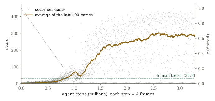Training curve: score per game and the average over 100 games, with ε Fig. 2: Score per game during training (including ε-exploration) and the average of the last 100 games. Dashed: the human reference score from the DQN paper. Dotted: ε.

Nothing happens for a long time. For the first 500 000 steps the average stays in single digits while ε is still high. Around one million steps, when ε reaches its floor, the score passes the human reference of 31.8 and shoots up to about 200 within the next 500 000 steps.
Plateau. From 2.5 million steps on the average of 100 games stays around 290, with single games up to 450.
Evaluation. The network after 3.2 million steps (12.8 million frames) scores 260 ± 107 over 10 games with ε = 0.05, between 105 and 388. The DQN paper reports 401 after 50 million frames.¹
Why not fully greedy. The emulator is deterministic. Played with ε = 0, the same network got stuck at 87 points: the ball settled into a path that never reached a brick, and 3000 steps passed without a point. The few random actions of ε = 0.05 are what breaks such loops, which is why the paper evaluates with it.
The action values are close together. In most states the four Q-values differ by only a few percent (Video 1). Over the next few steps one button rarely matters much, the ball is still far away. The differences that decide the game are small, so the estimates have to be precise.
Tunnels. The agent learned the classic strategy without being told: clear one side of the wall and let the ball bounce behind it. This also sidesteps the hardest part of the game, because the ball speeds up after the 4th and 12th hit and the paddle halves once the ball reaches the top wall.
The loss is not a progress measure. It jumps between minibatches, depending on whether a rare reward is in the batch, and after every target update. As the agent gets better its Q-values grow, and the loss often grows with them. The average score is what to watch, and the loss only has to stay finite.

The variance between games is large, and DQN can lose performance again late in training. The script overwrites one checkpoint every 100 000 steps, so a collapse would take the best network with it.

What ε-greedy cannot do

ε-greedy explores one step at a time: one random button, then greedy again. For Q-learning that is often enough, because a single deviation is exactly what $Q(s, a)$ measures: take $a$ once, then play well. Breakout is forgiving, since random play already hits a brick now and then. In games where the first reward needs a long, specific sequence of actions, such as Montezuma’s Revenge, DQN with ε-greedy scores close to zero. There one needs exploration that is extended in time or driven by curiosity.

Volodymyr Mnih, Koray Kavukcuoglu, David Silver, Andrei A. Rusu, Joel Veness, Marc G. Bellemare, Alex Graves, Martin Riedmiller, Andreas K. Fidjeland, Georg Ostrovski, Stig Petersen, Charles Beattie, Amir Sadik, Ioannis Antonoglou, Helen King, Dharshan Kumaran, Daan Wierstra, Shane Legg, Demis Hassabis. Human-level control through deep reinforcement learning. Nature 518, 529–533, 2015. doi:10.1038/nature14236 ↩ ↩²